---
title: "Lift charts and Lorenz curves"
description: "Does the model separate low risks from high risks? Lift charts, double lift charts, Lorenz curves and the Gini index for pure premium."
---
```{python}
#| include: false
import matplotlib.pyplot as plt
import numpy as np
import pandas as pd
from modelperf.metrics import deviance_metrics, exposure_bins, gini_index, lorenz_curve, regression_metrics, segment_table
from modelperf.models import TWEEDIE_POWER, pure_premium_predictions
from modelperf.plots import plot_lorenz, plot_segments, use_style
use_style()
p = pure_premium_predictions()
y, w = p["y"], p["w"]
models = ("GLM", "GBM")
mean = np.average(y, weights=w)
gini = {m: gini_index(y, p[m], w) for m in models}
d2 = {m: deviance_metrics(y, p[m], p["Null"], w, TWEEDIE_POWER)["D²"] for m in models}
```
**Question answered:** does the model separate low risks from high risks, and
is its prediction right for each risk segment?
The [deviance page](deviance.qmd) ended with D² values of about
`{python} f"{d2['GBM']:.1%}"`: individual claims are mostly chance, so any
average over individual errors is small. A pricing model is judged on
something else: whether the policies it calls expensive really cost more, *as a
group*, than the ones it calls cheap. Grouping averages away the noise. This
page covers the standard tools for that:
- the **lift chart**: actual against predicted, by decile of the prediction;
- the **double lift chart**: two models compared where they disagree;
- the **Lorenz curve** and the **Gini index**: one number for how well a
model separates risks.
## The lift chart
To draw a lift chart (also called a *quantile plot*):
1. sort the test policies by their predicted pure premium,
2. cut them into 10 groups (**deciles**) holding the same total exposure,
3. per decile, compare the exposure-weighted **average prediction** with the
**average actual** pure premium.
The deciles hold equal *exposure* rather than equal numbers of policies,
because pure premium is a rate per policy-year: a decile full of short policies
would hold far less information than its policy count suggests.
```{python}
#| label: fig-lift
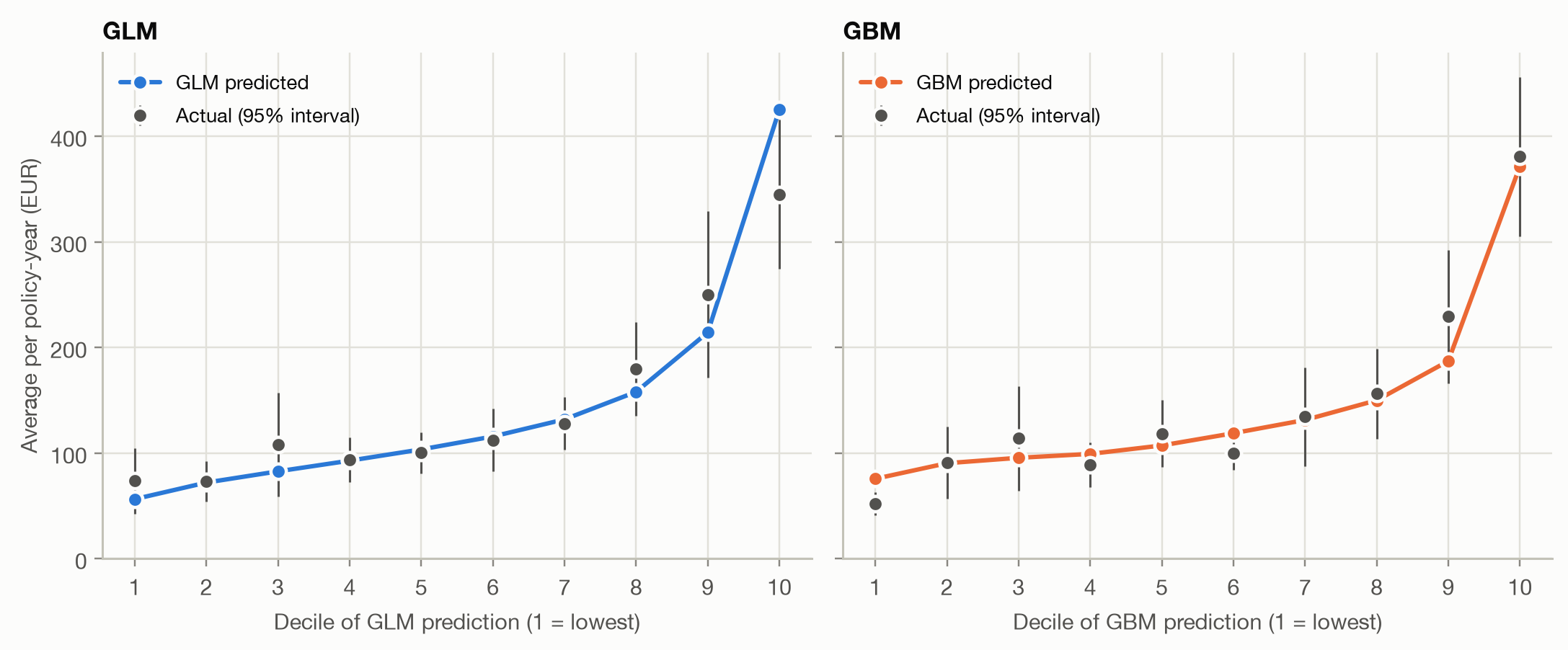
#| fig-cap: "Lift charts on the test set: average actual and predicted pure premium per decile of each model's prediction (deciles of equal exposure). Bars are 95% intervals for the actual average."
lift = {m: segment_table(y, {m: p[m]}, w, sort_by=p[m]) for m in models}
fig, axes = plt.subplots(1, 2, figsize=(10, 4.2), sharey=True)
for ax, m in zip(axes, models):
    plot_segments(lift[m], [m], ax=ax, xlabel=f"Decile of {m} prediction (1 = lowest)", title=m)
axes[1].set_ylabel("")
fig.tight_layout()
```
A good lift chart shows three things:
- **Monotonicity.** Actual cost should rise from decile to decile. Both models
get there broadly, with a few dips in the middle.
- **Spread.** The steeper the actual curve, the better the model separates risks.
The ratio of the top to the bottom decile is a common summary (the
'lift' that gives the chart its name).
- **Agreement.** The predicted line should run through the actual points. A
gap shows the predictions are off for that segment even when the overall
average is right: calibration, checked by group.
```{python}
#| label: tbl-lift
#| tbl-cap: "Summaries of the lift charts. Lift is the top decile's actual average divided by the bottom decile's (or by the overall average)."
pd.DataFrame({
    m: {
        "actual, decile 1 (EUR)": t.loc[1, "actual"],
        "actual, decile 10 (EUR)": t.loc[10, "actual"],
        "lift: decile 10 ÷ decile 1": t.loc[10, "actual"] / t.loc[1, "actual"],
        "lift: decile 10 ÷ overall": t.loc[10, "actual"] / mean,
        "predicted ÷ actual, decile 10": t.loc[10, m] / t.loc[10, "actual"],
    }
    for m, t in lift.items()
}).round(2)
```
```{python}
#| include: false
top_ratio = {m: lift[m].loc[10, m] / lift[m].loc[10, "actual"] for m in models}
spread = {m: lift[m].loc[10, "actual"] / lift[m].loc[1, "actual"] for m in models}
decile = exposure_bins(p["GBM"], w)
policies_per_decile = np.bincount(decile)
claims_per_decile = np.bincount(decile, weights=y > 0).astype(int)
```
The GBM's top decile costs `{python} f"{spread['GBM']:.1f}"` times its bottom
decile, against `{python} f"{spread['GLM']:.1f}"` times for the GLM. Where the
models differ most is the top decile: the GLM predicts
`{python} f"{top_ratio['GLM'] - 1:.0%}"` more than its riskiest policies
actually cost, while the GBM is within `{python} f"{abs(top_ratio['GBM'] - 1):.0%}"`.
The GLM's predictions are too extreme at the top, the regression-to-the-mean
pattern the [calibration page](../binary/calibration.qmd) described for
probabilities.
::: {.callout-note}
## Read the intervals before reading the dips
Each decile holds `{python} f"{policies_per_decile.min():,}"` to
`{python} f"{policies_per_decile.max():,}"` policies, but only
`{python} f"{claims_per_decile.min():,}"` to `{python} f"{claims_per_decile.max():,}"`
of them have a claim, and claim sizes vary enormously. The 95% intervals are
wide, so a dip such as the GBM's 4th decile is well within noise. Don't
redesign a model to remove a wiggle that the intervals cover.
:::
## The double lift chart
Two lift charts side by side are hard to compare: both look good, and their
deciles contain different policies. The **double lift chart** compares the two
models directly, on the policies where they **disagree**:
1. put both models on the same overall level (here: rescale each so its
average on the test set equals the actual average), so a difference in the
overall level doesn't look like a difference in segmentation;
2. sort the policies by the ratio GBM ÷ GLM, and cut them into deciles of equal
exposure;
3. per decile, compare the actual average with both models' averages.
Decile 1 holds the policies the GBM rates much lower than the GLM, decile 10
those it rates much higher. In the middle the models agree.
```{python}
#| code-fold: false
rebalanced = {m: p[m] * mean / np.average(p[m], weights=w) for m in models}
double = segment_table(y, rebalanced, w, sort_by=rebalanced["GBM"] / rebalanced["GLM"])
```
```{python}
#| label: fig-double-lift
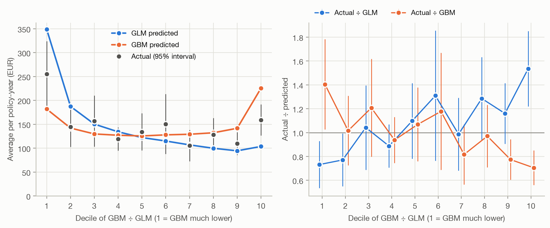
#| fig-cap: "Double lift chart, GBM against GLM. Left: average actual and predicted pure premium per decile of the ratio GBM ÷ GLM. Right: actual ÷ predicted for each model; 1 means the model's average is right for that decile."
xlabel = "Decile of GBM ÷ GLM (1 = GBM much lower)"
fig, axes = plt.subplots(1, 2, figsize=(10, 4.2))
plot_segments(double, models, ax=axes[0], xlabel=xlabel, legend_loc="upper center")
plot_segments(double, models, ax=axes[1], ratio=True, xlabel=xlabel)
fig.tight_layout()
```
```{python}
#| include: false
d1, d10 = double.loc[1], double.loc[10]
```
The left panel answers the question 'who is right where they disagree?' In
decile 1, the GLM predicts `{python} f"{d1['GLM']:.0f}"` EUR, the GBM
`{python} f"{d1['GBM']:.0f}"` EUR, and the actual average is
`{python} f"{d1['actual']:.0f}"` EUR. In decile 10, the GLM predicts
`{python} f"{d10['GLM']:.0f}"`, the GBM `{python} f"{d10['GBM']:.0f}"`, and the
actual average is `{python} f"{d10['actual']:.0f}"`. **Neither model wins:** in
both tails the truth lies between them.
The right panel shows the same comparison as actual ÷ predicted. The better
model is the one whose curve stays **flat at 1**. Insurers read this as a loss
ratio: if premiums were set by the GLM, actual ÷ GLM is the loss ratio each
segment would produce.
- **Actual ÷ GLM rises** from `{python} f"{d1['actual'] / d1['GLM']:.2f}"` to
`{python} f"{d10['actual'] / d10['GLM']:.2f}"`. The GBM finds policies the
GLM overprices (left) and underprices (right).
- **Actual ÷ GBM falls** from `{python} f"{d1['actual'] / d1['GBM']:.2f}"` to
`{python} f"{d10['actual'] / d10['GBM']:.2f}"`. The GLM finds mispricing in the
GBM just as well.
Each model knows something the other doesn't, and each overreacts where it
disagrees with the other. A curve that crosses 1 in the *opposite* direction
would mean the model is worse than useless where the two differ: its
deviations from the other model point the wrong way.
### What the double lift chart suggests: blend
When both models are partly right, a combination usually beats either. A
simple blend is the geometric mean of the two predictions (an average on the
log scale, which suits multiplicative pricing models):
```{python}
#| code-fold: false
blend = np.sqrt(rebalanced["GLM"] * rebalanced["GBM"])
blend *= mean / np.average(blend, weights=w)
```
```{python}
#| label: fig-double-lift-blend
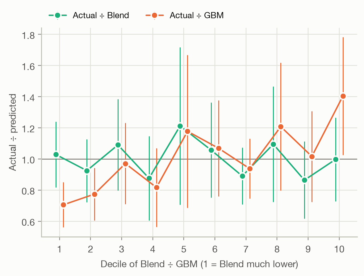
#| fig-cap: "Double lift chart, blend against GBM: actual ÷ predicted per decile of the ratio Blend ÷ GBM."
double_blend = segment_table(y, {"Blend": blend, "GBM": rebalanced["GBM"]}, w, sort_by=blend / rebalanced["GBM"])
ax = plot_segments(double_blend, ["Blend", "GBM"], ratio=True, xlabel="Decile of Blend ÷ GBM (1 = Blend much lower)")
ax.figure.set_size_inches(6, 4)
```
```{python}
#| label: tbl-blend
#| tbl-cap: "Gini index and D² (Tweedie, p = 1.9) of the two models and their blend on the test set."
#| code-fold: false
scores = {**{m: p[m] for m in models}, "Blend": blend}
pd.DataFrame({
    m: {"Gini": gini_index(y, s, w), "D²": deviance_metrics(y, s, p["Null"], w, TWEEDIE_POWER)["D²"]}
    for m, s in scores.items()
}).round(4)
```
Against the blend, the GBM's actual ÷ predicted swings away from 1 at both ends,
while the blend's stays near 1 within the noise: in this pairing, the blend
wins. The blend also has the highest Gini and D². Two caveats: the comparison
is on the test set the double lift chart was read from, so a blend chosen this
way should be confirmed on fresh data; and whether its improvement is larger
than sampling noise is a question for the [model-comparison page](../comparison/model-comparison.qmd).
## The Lorenz curve and the Gini index
The lift chart shows separation decile by decile. The **Lorenz curve** shows it
as one continuous curve:
1. sort the policies from the **lowest** to the **highest** prediction,
2. walk along the sorted list and plot the **share of total exposure** covered
so far (x-axis) against the **share of total claim cost** it contains
(y-axis).
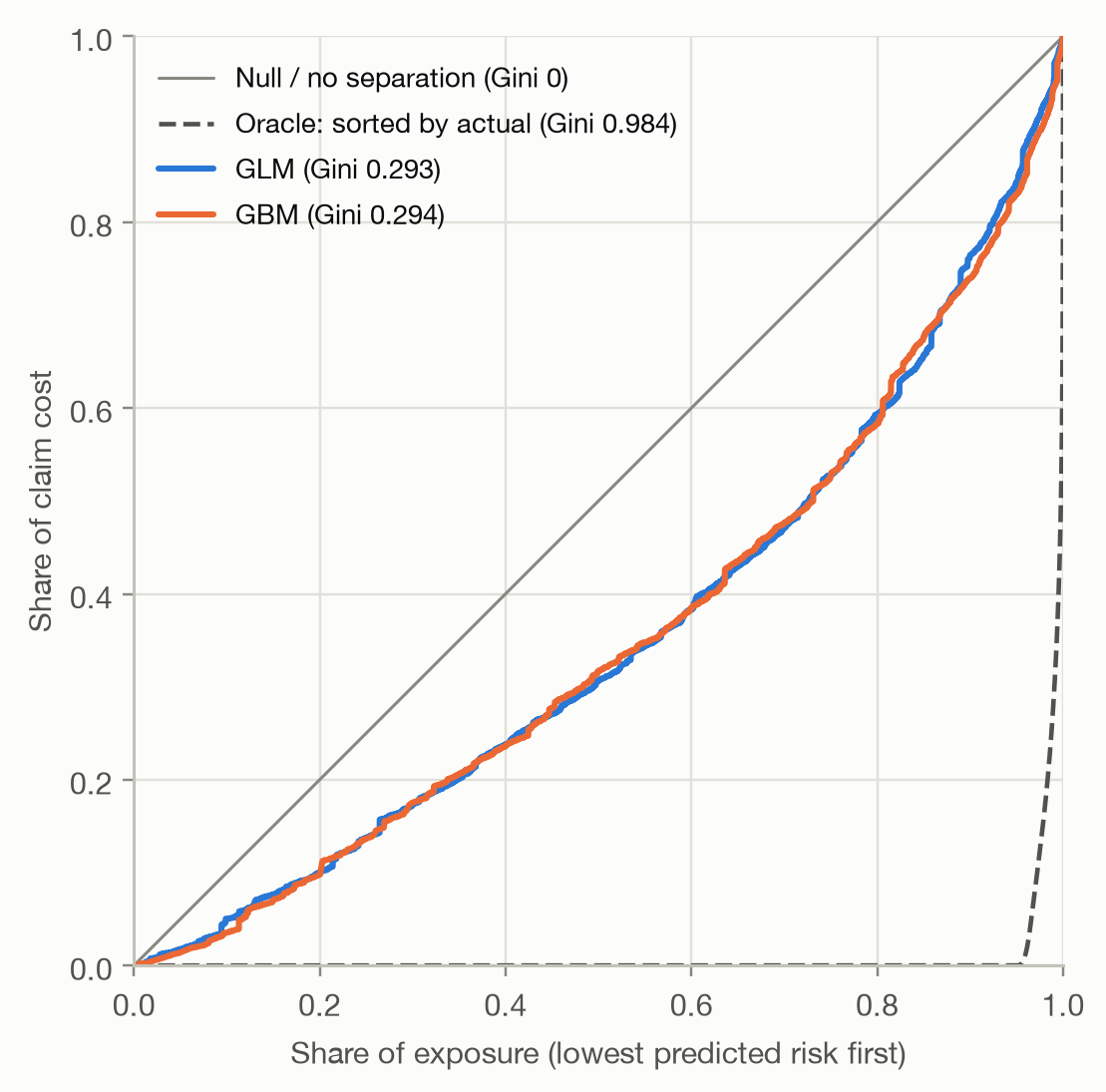
A model that can't separate risks (the Null model) gives the diagonal: the
first 30% of exposure carries 30% of the claim cost. A model that separates
well puts little claim cost into its low-risk policies, so its curve sags
below the diagonal. The **oracle** sorts by the actual outcome, the best
ranking possible.
```{python}
#| label: fig-lorenz
#| fig-cap: "Lorenz curves on the test set, policies sorted from lowest to highest prediction. The dashed curve sorts by the actual outcome."
ax = plot_lorenz(y, {m: p[m] for m in models}, w)
ax.figure.set_size_inches(5.5, 5.5)
```
```{python}
#| include: false
lc = lorenz_curve(y, p["GBM"], w)
half = np.interp(0.5, lc["exposure_share"], lc["loss_share"])
oracle = gini_index(y, y, w)
zero_share = np.average(y == 0, weights=w)
```
The GBM's lowest-risk half of the exposure carries only
`{python} f"{half:.0%}"` of the claim cost. The **Gini index** condenses the
curve into one number: twice the area between the diagonal and the curve,
$$
\text{Gini} = 1 - 2 \int_0^1 L(x)\,dx,
$$
where $L(x)$ is the share of claim cost in the lowest-predicted share $x$ of
the exposure. It is 0 for the Null model and grows the better the model ranks
the policies. The two models score `{python} f"{gini['GLM']:.3f}"` (GLM) and
`{python} f"{gini['GBM']:.3f}"` (GBM), a relative difference of
`{python} f"{gini['GBM'] / gini['GLM'] - 1:.1%}"`. On D² the GBM was
`{python} f"{d2['GBM'] / d2['GLM'] - 1:.0%}"` ahead, and its top-to-bottom
lift was much larger. The Gini weighs the whole ranking, while the lift ratio
looks only at the two extreme deciles, each resting on a few hundred claims. A
single decile ratio is a much noisier summary than the Gini.
The oracle's Gini of `{python} f"{oracle:.3f}"` is not a realistic target:
`{python} f"{zero_share:.0%}"` of the exposure had no claim at all, and only
hindsight can put those policies first. Some authors report a **normalized
Gini** (Gini ÷ oracle Gini), but the oracle mostly reflects how many policies
happened to have no claims, so it adds little here.
::: {.callout-note}
## Relation to the classification Gini
The [ROC page](../binary/roc-auc.qmd) defined Gini = 2·AUC − 1 for a binary
target. For a 0/1 outcome with equal weights, the Lorenz Gini equals
$(1 - \pi)(2 \cdot \text{AUC} - 1)$, where $\pi$ is the share of positives
(the tests in `tests/` check this). The factor $1 - \pi$ is the oracle's Gini:
dividing by it gives the normalized Gini, which equals 2·AUC − 1. Both measure
how well the model ranks. The Lorenz version extends the idea to outcomes that
aren't 0/1, such as claim cost, and to weighted observations.
:::
### What the Gini can't see
The Gini depends **only on the ranking**. Any transformation that keeps the
order of the predictions leaves it unchanged, however wrong the predictions
become:
```{python}
#| label: tbl-gini-blind
#| tbl-cap: "Three versions of the GBM with identical rankings. 'Squared' is GBM², rescaled to the same average, so its overall level is right but its spread is far too wide."
#| code-fold: false
squared = p["GBM"] ** 2 * np.average(p["GBM"], weights=w) / np.average(p["GBM"] ** 2, weights=w)
variants = {"GBM": p["GBM"], "2 × GBM": 2 * p["GBM"], "GBM squared": squared}
pd.DataFrame({
    name: {
        "Gini": gini_index(y, s, w),
        "D²": deviance_metrics(y, s, p["Null"], w, TWEEDIE_POWER)["D²"],
        "bias (EUR)": regression_metrics(y, s, w)["bias"],
    }
    for name, s in variants.items()
}).round(4)
```
Doubling every prediction, or squaring them, keeps the Gini exactly the same.
D² drops below 0 (worse than predicting the average for everyone), and a lift
chart would show the gap at once. So:
- **Never use the Gini alone.** Pair it with a lift chart or a calibration
check, and with the deviance.
- **Don't compare Ginis across portfolios or years.** Like AUC, the Gini
depends on how heterogeneous the population is: a portfolio with more varied
risks gives a higher Gini for an equally good model.
- **Small differences are noise.** The GLM and GBM differ by
`{python} f"{gini['GBM'] - gini['GLM']:.3f}"`, far less than the test-set
variability of a Gini on data this noisy. Testing such differences is the
subject of the [model-comparison page](../comparison/model-comparison.qmd).
## Which tool for which question
| Tool | Answers | Watch out for |
|---|---|---|
| Lift chart | Does cost rise with the prediction, and does the prediction match per segment? | noisy deciles: read the intervals |
| Double lift chart | Where two models disagree, which is right? | rebalance both models to the same level first |
| Lorenz curve / Gini | How well does the model rank risks, in one number? | blind to calibration and level; not comparable across portfolios |
| Deviance / D² | How good are the individual predictions, ranking and level together? | small values are normal; hard to interpret alone |
The tools complement each other: the Gini and the lift spread measure
**ranking**, the agreement in the lift chart measures **calibration by
segment**, the double lift chart **compares** two candidate models, and the
deviance checks both ranking and level at once.
## Takeaways
- With noisy outcomes, judge a pricing model on **groups**: deciles of equal
exposure average away the noise that dominates individual-level metrics.
- A **lift chart** should rise monotonically, be steep, and have predictions
that run through the actual points. Here the GLM overpredicts its top decile
by `{python} f"{top_ratio['GLM'] - 1:.0%}"`.
- A **double lift chart** compares two models where they disagree. Here each
model finds mispricing in the other, and a simple **blend** beats both.
- The **Gini index** summarizes the Lorenz curve: `{python} f"{gini['GLM']:.3f}"`
(GLM) against `{python} f"{gini['GBM']:.3f}"` (GBM). It measures ranking only,
so a badly miscalibrated model can have the same Gini as a good one.