---
title: "Calibration and proper scoring rules"
description: "Do predicted probabilities match observed frequencies? Reliability diagrams, calibration slope, Brier score, log loss and the Murphy decomposition."
---
```{python}
#| include: false
import matplotlib.pyplot as plt
import numpy as np
import pandas as pd
from scipy.special import expit, logit
from modelperf.data import train_test
from modelperf.metrics import (
auc_rank,
calibration_intercept_slope,
expected_calibration_error,
murphy_decomposition,
)
from modelperf.models import binary_predictions
from modelperf.plots import plot_reliability, use_style
use_style()
b = binary_predictions()
y = b["y"]
rate = y.mean()
```
**Question answered:** when the model says 10%, does the event happen about
10% of the time?
The [ROC page](roc-auc.qmd) ended with a warning: AUC only measures
*ranking*. A model can rank perfectly and still predict probabilities that are
far off. Whenever the probabilities themselves are used, for a premium, an
expected cost, a capital estimate or the
[cost-based threshold](confusion-matrix.qmd#choosing-a-threshold), they must
also be **calibrated**.
## What calibration means
A model is calibrated if, among all cases that receive prediction $\hat p$,
the event happens with frequency $\hat p$:
$$
P(Y = 1 \mid \hat p = p) = p \quad \text{for all } p.
$$
Calibration and discrimination are separate properties:
- Always predicting the overall claim rate (the Null model) is **perfectly
calibrated but has no discrimination**.
- Dividing every GBM prediction by 10 keeps the **discrimination but ruins
calibration**.
A good model needs both.
## Calibration in the large
The simplest check: is the average prediction equal to the observed rate?
```{python}
#| label: tbl-in-the-large
#| tbl-cap: "Average predicted probability and observed claim rate on the test set."
pd.DataFrame({
    "Average prediction": {m: b[m].mean() for m in ("Null", "GLM", "GBM")},
    "Observed rate": {m: rate for m in ("Null", "GLM", "GBM")},
}).round(4)
```
All three are close to the observed `{python} f"{rate:.2%}"`. This check is
necessary but far from sufficient: a model can be right on average while too
high for low risks and too low for high risks, and these errors cancel out.
## Reliability diagrams
A **reliability diagram** plots the observed rate against the predicted
probability. A calibrated model follows the diagonal. Points above the diagonal
mean the model predicts **too low** there, points below mean **too high**.
### The classic version: binning
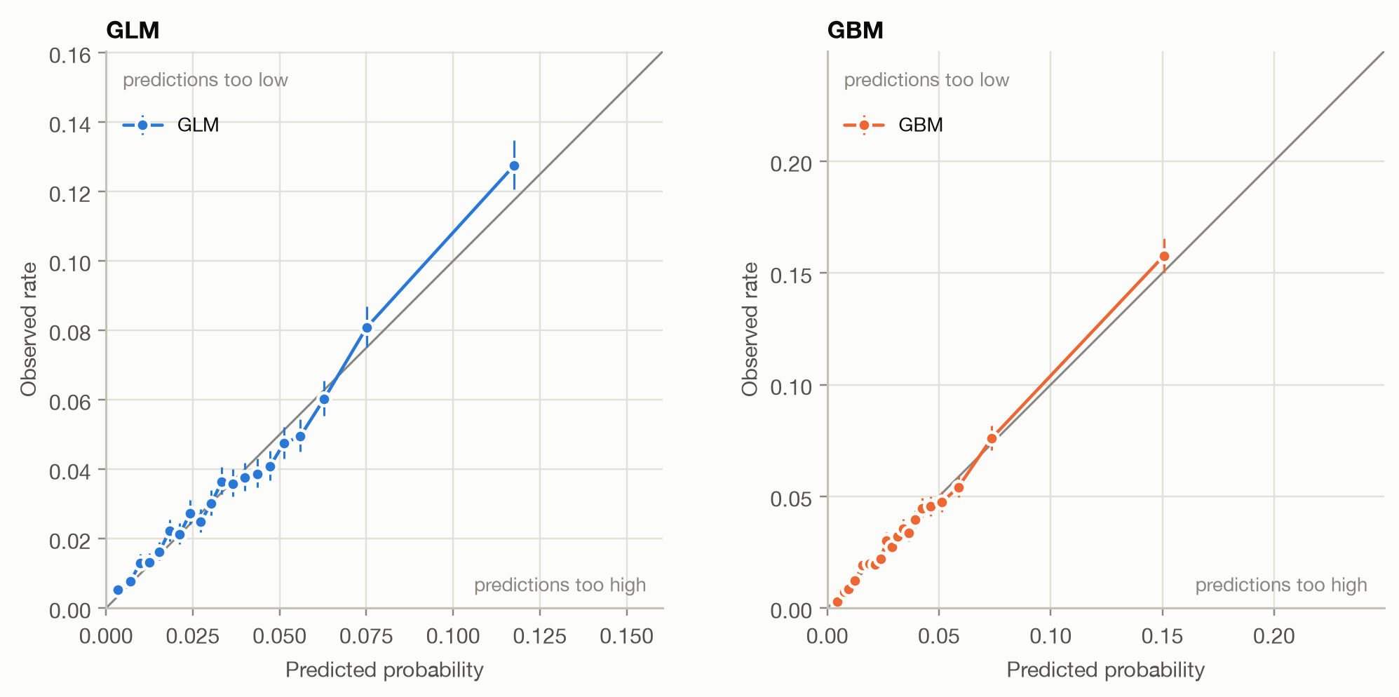
The usual recipe sorts the cases by prediction, splits them into bins (here 20
bins with equal numbers of policies), and plots each bin's average prediction
against its observed claim rate:
```{python}
#| label: fig-reliability-bins
#| fig-cap: "Binned reliability diagrams: 20 bins of equal size, with 95% confidence intervals for the observed rate."
fig, axes = plt.subplots(1, 2, figsize=(9.5, 4.5))
for ax, m in zip(axes, ("GLM", "GBM")):
    plot_reliability(y, {m: b[m]}, ax=ax, method="bins", title=m)
fig.tight_layout()
```
Both models stay close to the diagonal over most of the range. Most policies
have a predicted probability below 10%, so the bins are packed there and
sparse above. The few high-risk bins carry wide confidence intervals.
### The problem with bins
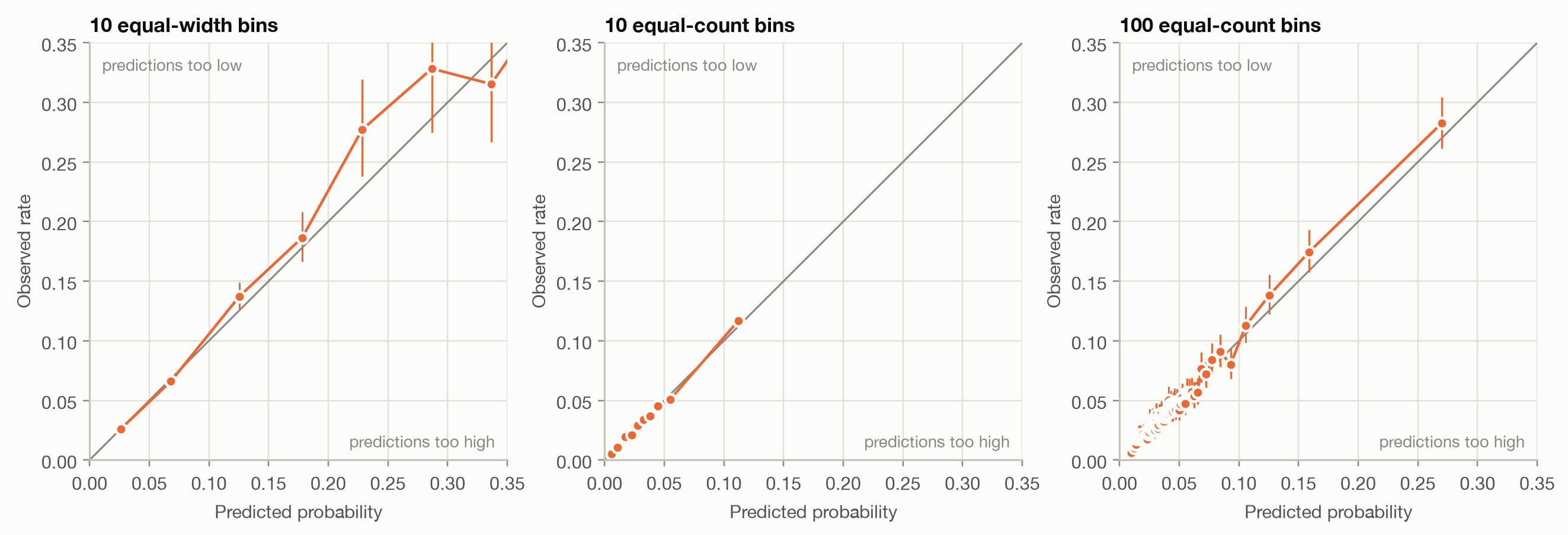
The picture depends on how the bins are chosen, and there's no right choice.
The same GBM with different binnings:
```{python}
#| label: fig-binning
#| fig-cap: "The GBM's reliability diagram under three binning choices."
fig, axes = plt.subplots(1, 3, figsize=(12, 4.2))
for ax, (n, strategy) in zip(axes, [(10, "uniform"), (10, "quantile"), (100, "quantile")]):
    plot_reliability(y, {"GBM": b["GBM"]}, ax=ax, method="bins", n_bins=n, strategy=strategy,
                     max_p=0.35, title=f"{n} {'equal-width' if strategy == 'uniform' else 'equal-count'} bins")
    ax.get_legend().remove()
fig.tight_layout()
```
Equal-width bins put nearly all policies in the first two bins and leave the
rest nearly empty. Few equal-count bins hide any detail at the high end. Many
bins turn the diagram into noise. Summary statistics built on bins inherit the
problem. The **expected calibration error** (ECE), the share-weighted average
gap between bin prediction and bin rate, changes with the binning:
```{python}
#| label: tbl-ece
#| tbl-cap: "Expected calibration error of the same predictions under different binnings."
settings = [(10, "uniform"), (20, "uniform"), (5, "quantile"), (10, "quantile"), (20, "quantile"), (100, "quantile")]
pd.DataFrame({
    f"{n} {'equal-width' if s == 'uniform' else 'equal-count'}": {
        m: expected_calibration_error(y, b[m], n, s) for m in ("GLM", "GBM")
    }
    for n, s in settings
}).T.round(5)
```
```{python}
#| include: false
ece = {n: expected_calibration_error(y, b["GBM"], n, "quantile") for n in (5, 100)}
```
With 100 bins, the GBM's ECE is `{python} f"{ece[100] / ece[5]:.0f}"` times
larger than with 5 bins. That's not because the model got worse: smaller bins
simply contain more sampling noise. ECE values are only comparable at the
same binning, and even then mostly measure noise when bins are small.
### The modern version: CORP
The **CORP** approach (consistent, optimally binned, reproducible;
Dimitriadis, Gneiting and Jordan, 2021) replaces hand-chosen bins with
**isotonic regression**. It finds the best *non-decreasing* step function
mapping predictions to observed outcomes, using the pool-adjacent-violators
(PAV) algorithm. In effect, the data chooses the bins: adjacent predictions
are merged exactly where their outcomes don't support a higher rate.
- **No tuning:** no bin count or bin edges to choose, so the result is
reproducible.
- **Consistent:** with more data, the curve converges to the true calibration
curve.
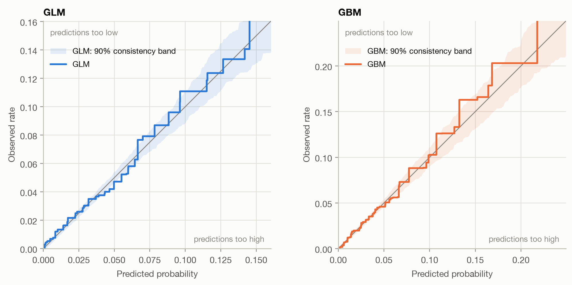
- **Uncertainty built in:** simulating outcomes *from the model's own
probabilities* shows how much a perfectly calibrated model's curve wobbles by
chance. The 90% range of these simulations is the **consistency band**.
Where the observed curve leaves the band, the miscalibration is real.
```{python}
#| label: fig-corp
#| fig-cap: "CORP reliability diagrams with 90% consistency bands (200 simulations each)."
fig, axes = plt.subplots(1, 2, figsize=(9.5, 4.5))
for ax, m in zip(axes, ("GLM", "GBM")):
    plot_reliability(y, {m: b[m]}, ax=ax, method="corp", band=True, title=m)
fig.tight_layout()
```
Both curves follow the diagonal closely where most policies are, below about
6%. Above that, both tend to run above the diagonal, and the GLM's curve leaves
its band several times. Both models under-predict their highest risks, the
GLM more clearly. The [segment analysis](#calibration-within-segments) below
shows where this comes from. In practice, the CORP diagram should be the
default, and binned diagrams kept for audiences used to them.
## Calibration intercept and slope
Two numbers summarize the most common patterns of miscalibration. Fit a
logistic regression of the outcome on the model's logit,
$$
\operatorname{logit} P(Y = 1) = a + b \cdot \operatorname{logit}(\hat p),
$$
and read off:
| Statistic | Ideal | Meaning when off |
|---|---|---|
| **Calibration intercept** $a$ (with $b$ fixed at 1) | 0 | > 0: predictions too low on average; < 0: too high |
| **Calibration slope** $b$ | 1 | < 1: predictions **too extreme** (too spread out, typical of overfitting); > 1: **too timid** (not spread out enough, typical of over-regularization) |
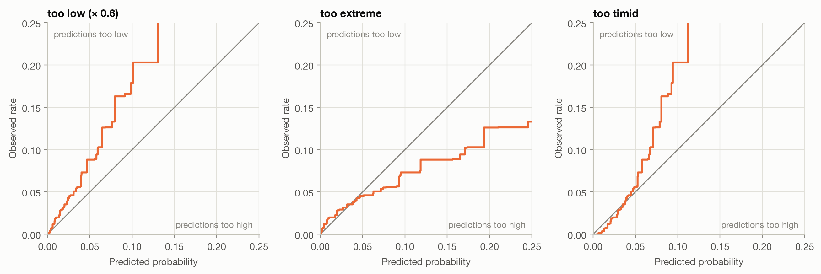
To see these patterns, we distort the GBM's predictions in three ways:
```{python}
#| code-fold: false
center = logit(rate)
variants = {
    "GBM": b["GBM"],
    "too low (× 0.6)": 0.6 * b["GBM"],
    "too extreme": expit(center + 1.6 * (logit(b["GBM"]) - center)),
    "too timid": expit(center + 0.6 * (logit(b["GBM"]) - center)),
}
```
```{python}
#| label: fig-patterns
#| fig-cap: "CORP reliability curves of three distorted versions of the GBM."
fig, axes = plt.subplots(1, 3, figsize=(12, 4.2))
for ax, name in zip(axes, list(variants)[1:]):
    plot_reliability(y, {name: variants[name]}, ax=ax, max_p=0.25, title=name,
                     colors={name: "#eb6834"})
    ax.get_legend().remove()
fig.tight_layout()
```
```{python}
#| label: tbl-slope
#| tbl-cap: "Calibration intercept, slope and AUC of the models and the distorted variants."
rows = {m: b[m] for m in ("GLM", "GBM")} | {k: v for k, v in variants.items() if k != "GBM"}
pd.DataFrame({
    k: pd.concat([calibration_intercept_slope(y, v), pd.Series({"AUC": auc_rank(y, v)})])
    for k, v in rows.items()
}).T.round(3)
```
- The **GLM and GBM** have intercepts near 0 and slopes near 1: well
calibrated overall.
- **Too low** shows a positive intercept: the curve runs above the diagonal
everywhere.
- **Too extreme** has a slope below 1: low risks predicted too low, high risks
too high. The curve is flatter than the diagonal. This is what an overfitted
model looks like on new data.
- **Too timid** has a slope above 1: the curve is steeper than the diagonal.
- The **AUC is identical** for all GBM variants. None of these problems
is visible in ranking metrics.
## Proper scoring rules
Calibration plots diagnose. To *compare* models with a single number that
rewards both calibration and discrimination, use a **proper scoring rule**.
It's a score whose expected value is best when the predicted probability
equals the true probability, so no forecaster can improve their expected score
by reporting anything other than what they believe. The two standard ones,
lower is better for both:
$$
\text{Brier score} = \frac{1}{n}\sum_{i} (\hat p_i - y_i)^2,
\qquad
\text{log loss} = -\frac{1}{n}\sum_{i} \big[ y_i \log \hat p_i + (1 - y_i)\log(1 - \hat p_i) \big].
$$
- **Brier score**: squared error on probabilities. It's bounded and robust,
but small differences are hard to see when events are rare.
- **Log loss**: the negative log-likelihood, and exactly what logistic
regression and the GBM were trained on. It punishes confident wrong
predictions without limit: predicting 0.1% for a policy that does have a
claim costs far more than predicting 10% for one that doesn't.
Accuracy, F1 and AUC are **not** proper scoring rules. Accuracy and F1 only see
which side of a threshold a prediction falls on, and AUC only sees ranking. A
model can improve on them while its probabilities get worse.
### The Murphy decomposition
A raw score is hard to interpret on its own. The CORP decomposition splits any
proper score exactly into three parts:
$$
\text{score} = \underbrace{\text{MCB}}_{\text{miscalibration}} - \underbrace{\text{DSC}}_{\text{discrimination}} + \underbrace{\text{UNC}}_{\text{uncertainty}}.
$$
- **UNC**: the score of the Null model, i.e. how hard the problem is. It's the
same for every model on the same data.
- **DSC**: how much the score improves when the predictions are optimally
recalibrated (isotonic regression), compared with the Null model. It
depends only on the *ranking*, like AUC. Higher is better.
- **MCB**: how much worse the actual predictions score than their
recalibrated version: the price paid for miscalibration. Lower is better.
```{python}
#| label: tbl-murphy
#| tbl-cap: "Murphy decomposition of the log loss. The two last rows are the order-preserving transformations from the ROC page."
cases = {m: b[m] for m in ("Null", "GLM", "GBM")} | {"GBM / 10": b["GBM"] / 10, "GBM ^ 0.2": b["GBM"] ** 0.2}
murphy = pd.DataFrame({k: murphy_decomposition(y, v, "log loss") for k, v in cases.items()}).T
murphy.round(5)
```
```{python}
#| include: false
gbm_glm_dsc = murphy.loc["GBM", "DSC"] / murphy.loc["GLM", "DSC"] - 1
```
The table answers *why* one model scores better than another:
- The **GBM beats the GLM through discrimination**: its DSC is
`{python} f"{gbm_glm_dsc:.0%}"` higher, while both have very small MCB.
- The two transformed GBMs have **exactly the GBM's DSC**: they rank the same.
All their extra loss is miscalibration.
- The **Null model** has DSC 0 and MCB 0: calibrated, but no discrimination.
The same table for the Brier score (try `murphy_decomposition(y, p, "Brier")`)
tells the same story. Use the decomposition whenever two models are
compared on a scoring rule: it separates 'ranks better' from 'is better
calibrated'.
## Calibration within segments
Overall calibration can hide miscalibration in subgroups, and subgroups are
often what matters, such as tariff cells, customer segments or regions.
Insurers check this with the **actual-to-expected (A/E) ratio**: observed
claims divided by predicted claims, per segment. A/E above 1 means the model
predicts too low for that segment.
```{python}
#| label: tbl-segments
#| tbl-cap: "Actual-to-expected ratio by bonus-malus level (test set)."
test = train_test().test
segment = pd.cut(test["BonusMalus"], [0, 50, 60, 80, 100, 250],
                 labels=["50 (best)", "51–60", "61–80", "81–100", "> 100 (malus)"])
df = b.assign(segment=segment.to_numpy())
grouped = df.groupby("segment", observed=True)
ae = pd.DataFrame({
    "Policies": grouped.size(),
    "Observed rate": grouped["y"].mean(),
    "A/E GLM": grouped["y"].sum() / grouped["GLM"].sum(),
    "A/E GBM": grouped["y"].sum() / grouped["GBM"].sum(),
})
ae.round(3)
```
```{python}
#| include: false
ae_malus = ae.loc["> 100 (malus)"]
```
The GLM is calibrated overall but not across bonus-malus levels: its A/E
ratios range from `{python} f"{ae['A/E GLM'].min():.2f}"` to
`{python} f"{ae['A/E GLM'].max():.2f}"`. For policyholders with a malus, it
predicts `{python} f"{ae_malus['A/E GLM'] - 1:.0%}"` fewer claims than
actually occur, while in the 81–100 band it predicts too many. The errors
cancel out in the overall average. The GLM uses a single log-linear effect for
bonus-malus, which is too rigid for the real relationship. The GBM stays
within a few percent in every segment. A table like this points directly to
the feature that needs a better specification.
::: {.callout-tip}
## Fixing miscalibration
If ranking is good but probabilities are off, a model can be **recalibrated**
by mapping its predictions through a fitted function:
- **Platt scaling** (logistic): fit the intercept and slope above, apply them.
Few parameters, robust, fixes the common patterns.
- **Isotonic regression**: the CORP curve itself. Flexible, but needs plenty
of data and produces step-shaped probabilities.
Fit the recalibration on data that wasn't used to train the model, and
evaluate on yet another set (scikit-learn: `CalibratedClassifierCV`). A
monotone recalibration leaves the ranking, and therefore AUC and DSC,
essentially unchanged. It only removes MCB.
:::
## Takeaways
- **Calibration** asks whether predicted probabilities match observed
frequencies. It's separate from discrimination, and AUC can't see it.
- Prefer **CORP reliability diagrams** with consistency bands over binned
diagrams. Bins and the ECE depend on arbitrary choices.
- **Calibration slope** < 1 signals predictions that are too extreme
(overfitting), > 1 too timid. The **intercept** shows systematic over- or
under-prediction.
- Compare models with **proper scoring rules** (log loss, Brier), and use the
**Murphy decomposition** to see whether a difference comes from
discrimination or calibration.
- Check calibration **within segments** (A/E ratios). Overall calibration can
hide large errors in the groups that matter.