---
title: "Error metrics: bias, MAE, RMSE and R²"
description: "How far off are the predictions? The standard metrics, what each one rewards, and where they break."
---
```{python}
#| include: false
import matplotlib.pyplot as plt
import numpy as np
import pandas as pd
from modelperf.metrics import regression_metrics
from modelperf.models import housing_predictions, pure_premium_predictions
from modelperf.plots import METRIC_COLORS, INK_SECONDARY, plot_actual_vs_predicted, plot_residuals, use_style
use_style()
h = housing_predictions()
y = h["y"]
```
**Question answered:** how far are the predictions from the actual values, on
average?
We start with **California Housing** (median house value per district, in
units of 100,000 USD), a target with a strong signal where these metrics
behave as textbooks describe. At the end, we apply them to **pure premium**
and watch them break.
## The four basic metrics
With errors $e_i = \hat y_i - y_i$ over $n$ test cases:
| Metric | Formula | Unit | Question it answers |
|---|---|---|---|
| Bias (mean error) | $\frac{1}{n}\sum e_i$ | target | Is the model systematically too high or too low? |
| MAE (mean absolute error) | $\frac{1}{n}\sum \lvert e_i \rvert$ | target | How large is a typical error? |
| RMSE (root mean squared error) | $\sqrt{\frac{1}{n}\sum e_i^2}$ | target | How large are errors, with big ones weighted more? |
| R² (coefficient of determination) | $1 - \frac{\sum e_i^2}{\sum (y_i - \bar y)^2}$ | none | What share of the variance does the model explain? |
With weights $w_i$ (as for pure premium, weighted by exposure), each sum
becomes a weighted sum and $n$ becomes $\sum w_i$.
```{python}
#| label: tbl-housing-metrics
#| tbl-cap: "Test-set error metrics on California Housing (units of 100,000 USD)."
#| code-fold: false
pd.DataFrame({m: regression_metrics(y, h[m]) for m in ("Null", "GLM", "GBM")}).round(3)
```
```{python}
#| include: false
hm = {m: regression_metrics(y, h[m]) for m in ("Null", "GLM", "GBM")}
usd = lambda v: f"{v * 100_000:,.0f} USD"
```
Reading the table:
- **Bias** is close to zero for all models. That's expected on data like the
training data: least squares fits reproduce the mean. Bias becomes
interesting once the data shifts: a growing bias is one of the first signs
of drift (covered on a later page).
- The GBM's typical error (MAE) is `{python} usd(hm["GBM"]["MAE"])`, against
`{python} usd(hm["GLM"]["MAE"])` for the GLM and
`{python} usd(hm["Null"]["MAE"])` for always predicting the mean.
- **RMSE is always at least as large as MAE.** The gap grows with the share of
large errors: squaring makes a single error of 3 count as much as nine
errors of 1.
- **R²** compares the squared error with that of the Null model: the GBM
removes `{python} f"{hm['GBM']['R²']:.0%}"` of the Null model's squared
error, the GLM `{python} f"{hm['GLM']['R²']:.0%}"`.
## What MAE and RMSE reward
MAE and RMSE don't just weigh errors differently, they reward **different
predictions**:
- **Squared error is minimized by the mean.** A model trained or selected on
RMSE learns the conditional *mean* of the target.
- **Absolute error is minimized by the median.** A model selected on MAE
learns the conditional *median*.
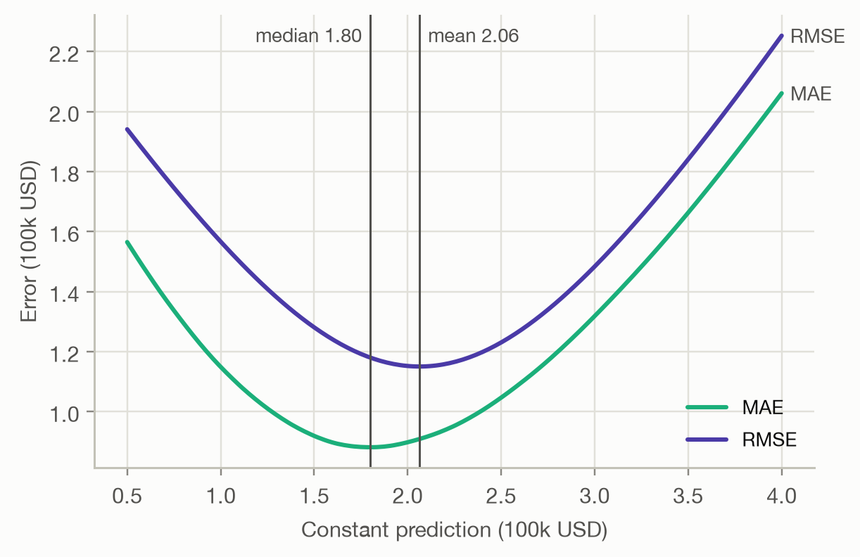
For a symmetric target the two coincide. For a skewed target, such as house
prices, claim costs or incomes, they don't. Scoring every *constant*
prediction shows this:
```{python}
#| label: fig-constant
#| fig-cap: "MAE and RMSE of predicting the same constant value for every district."
c = np.linspace(0.5, 4.0, 200)
mae = [np.mean(np.abs(y - v)) for v in c]
rmse = [np.sqrt(np.mean((y - v) ** 2)) for v in c]

fig, ax = plt.subplots(figsize=(6, 3.8))
for values, name, color in [(mae, "MAE", METRIC_COLORS[0]), (rmse, "RMSE", METRIC_COLORS[1])]:
    ax.plot(c, values, color=color, label=name)
    ax.annotate(name, (c[-1], values[-1]), xytext=(4, 0), textcoords="offset points",
                va="center", fontsize=9, color=INK_SECONDARY)
for stat, value, side in [("median", y.median(), -1), ("mean", y.mean(), 1)]:
    ax.axvline(value, color=INK_SECONDARY, linewidth=1)
    ax.annotate(f"{stat} {value:.2f}", (value, 1), xycoords=("data", "axes fraction"),
                xytext=(4 * side, -4), textcoords="offset points", va="top",
                ha="left" if side > 0 else "right", fontsize=9, color=INK_SECONDARY)
ax.set(xlabel="Constant prediction (100k USD)", ylabel="Error (100k USD)")
ax.legend(loc="lower right")
```
The MAE curve bottoms out at the median, the RMSE curve at the mean. So
choosing a metric is choosing **what the model should predict**. For pricing,
where the average cost must be covered, the mean is the right target and
squared-error-type metrics are the right family. MAE answers a different
question.
::: {.callout-warning}
## MAPE and other relative errors
The mean absolute percentage error, $\frac{1}{n}\sum \lvert e_i / y_i \rvert$,
is popular because it is unit-free. It is undefined when $y_i = 0$, explodes
when $y_i$ is small, and penalizes over-prediction more than
under-prediction, which pushes models to predict too low. Use it only for
targets well away from zero, and never for pure premium.
:::
## Looking at the errors
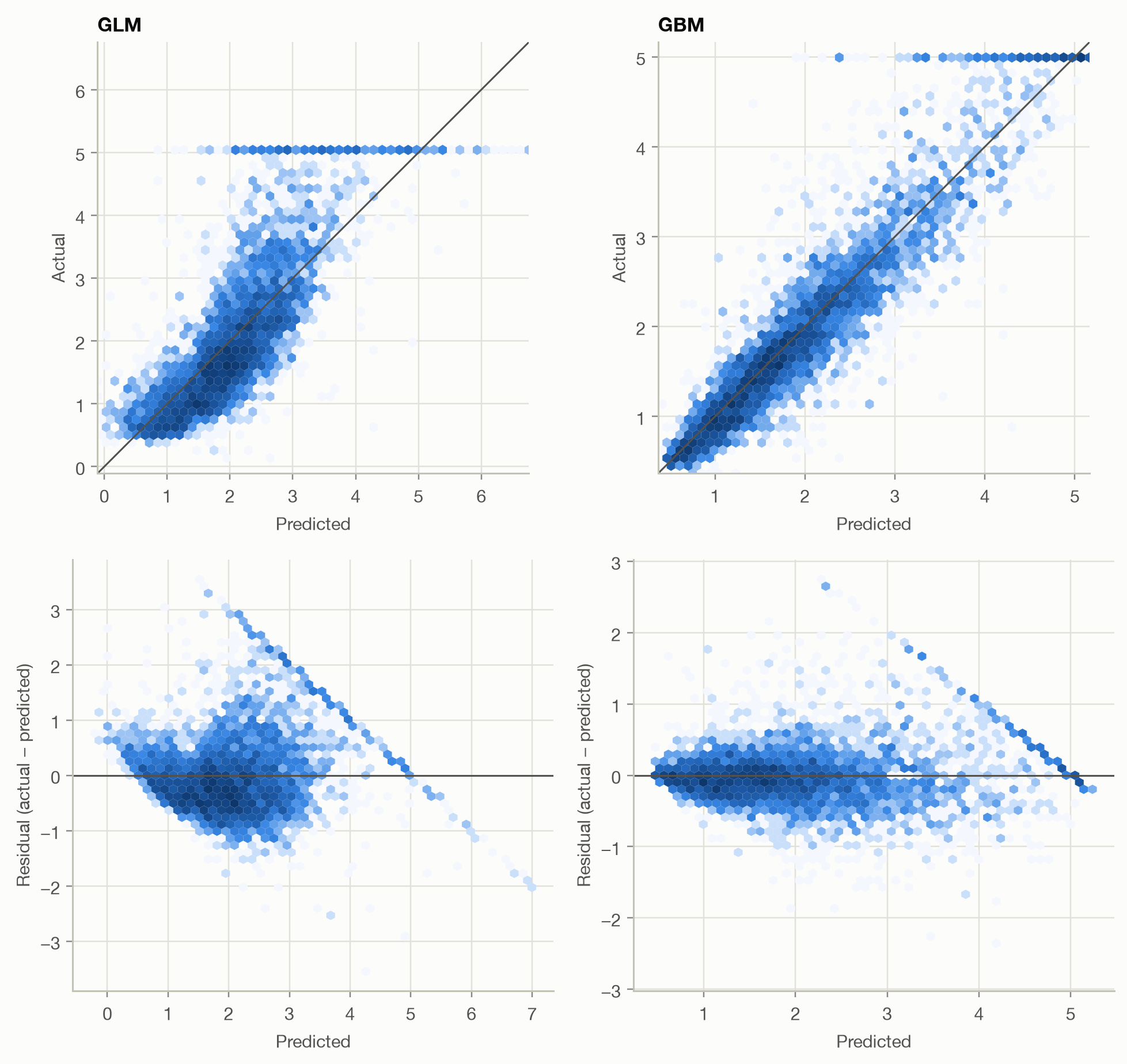
A single number hides *where* a model errs. Two plots do most of the work:
- **actual vs predicted**: points should scatter evenly around the diagonal,
- **residuals vs predicted**: residuals should scatter evenly around zero,
with no trend, no fan shape and no visible structure.
```{python}
#| label: fig-housing-diagnostics
#| fig-cap: "Actual vs predicted (top; the diagonal marks perfect prediction) and residuals vs predicted (bottom) for the GLM and the GBM. Color shows the number of districts per hexagon, on a log scale."
#| fig-height: 8
fig, axes = plt.subplots(2, 2, figsize=(9, 8.5))
for col, m in enumerate(("GLM", "GBM")):
    plot_actual_vs_predicted(y, h[m], ax=axes[0, col], title=m)
    plot_residuals(y, h[m], ax=axes[1, col])
fig.tight_layout()
```
```{python}
#| include: false
capped = f"{(y >= 5).mean():.1%}"
glm_outside = f"{((h['GLM'] > 5) | (h['GLM'] < 0)).mean():.1%}"
```
Three things stand out, none of which the metrics table shows:
1. **A horizontal line at 5.0** (a diagonal stripe in the residual plots).
`{python} capped` of districts have a value of exactly 5.0, because values
were capped when the data was collected. The true values are higher, so the
errors there are partly an artifact of the data, not of the model.
2. **The GLM's residuals trend downward.** It under-predicts cheap districts
and over-predicts expensive ones: the relationship isn't linear, and a
linear model can't bend to follow it. It also predicts outside the possible
range for `{python} glm_outside` of districts (above the cap or below zero).
3. **The GBM's residuals are tighter and centered on zero across the whole
range**, consistent with its lower RMSE, but they widen for expensive
districts. The errors are larger where values are larger, which is common
for prices and amounts.
## Where these metrics break: pure premium
Now apply the same metrics to pure premium, weighted by exposure. We add one
more 'model': predicting **0 for every policy**.
```{python}
#| label: tbl-pp-metrics
#| tbl-cap: "Exposure-weighted error metrics for pure premium (EUR per policy-year)."
#| code-fold: false
p = pure_premium_predictions()
preds = {m: p[m] for m in ("Null", "GLM", "GBM")} | {"Always 0": np.zeros(len(p))}
pd.DataFrame({m: regression_metrics(p["y"], v, p["w"]) for m, v in preds.items()}).round(4)
```
```{python}
#| include: false
pm = {m: regression_metrics(p["y"], v, p["w"]) for m, v in preds.items()}
```
The results are strange:
- **'Always 0' has the best MAE** (`{python} f"{pm['Always 0']['MAE']:.0f}"`
against `{python} f"{pm['GBM']['MAE']:.0f}"` for the GBM). Most policies
have no claim, so the median pure premium is 0, and MAE rewards the median.
A pricing model that charges nothing would win on MAE.
- **RMSE is nearly identical for all models** (about
`{python} f"{pm['GBM']['RMSE']:,.0f}"`). It's dominated by a few huge
claims spread over short exposures, which no model can predict.
- **R² is about 0.0005 for both models**: practically zero, even though, as
the next pages show, both models clearly separate low and high risks.
The problem isn't the models. These metrics assume errors of similar size
everywhere, and for insurance targets that assumption fails badly: most
outcomes are exactly zero, the rest vary enormously, and the variance grows
with the expected value. Such targets need a loss that matches their
distribution: the [deviance](deviance.qmd).
## Takeaways
- **Bias** checks systematic over- or under-prediction; **MAE** and **RMSE**
give the typical error size in the target's unit; **R²** compares with the
Null model.
- Choosing a metric chooses **what the model should predict**: RMSE rewards
the mean, MAE the median.
- **Plot the residuals.** Capped data, non-linear effects and growing error
variance stay invisible in summary metrics.
- For zero-heavy, skewed targets such as pure premium, MAE, RMSE and R² are
**misleading**. Use deviance and ranking-based measures instead.