---
title: "Deviance and D²"
description: "Error metrics that match the target's distribution: the right yardstick for insurance targets."
---
```{python}
#| include: false
import matplotlib.pyplot as plt
import numpy as np
import pandas as pd
from modelperf.metrics import deviance_metrics, regression_metrics, tweedie_deviance
from modelperf.models import TWEEDIE_POWER, pure_premium_predictions
from modelperf.plots import METRIC_COLORS, INK_SECONDARY, use_style
use_style()
p = pure_premium_predictions()
y, w = p["y"], p["w"]
```
**Question answered:** how well do the predictions fit, measured in a way that
respects the target's distribution?
The [previous page](error-metrics.qmd) ended with MAE, RMSE and R² failing on
pure premium. This page introduces the metric the models were actually trained
on: the **deviance**.
## Why squared error doesn't fit
Squared error treats an error of 100 EUR the same everywhere. That makes sense
when every observation is equally noisy. For insurance targets, the noise
grows with the expected value: a risk expected to cost 1,000 EUR a year varies
far more than one expected to cost 50 EUR. In the Tweedie family of
distributions, used for such targets, this is explicit:
$$
\operatorname{Var}(Y) = \phi \, \mu^{p},
$$
where $\mu$ is the expected value, $\phi$ a dispersion parameter, and the
**power** $p$ describes how fast the variance grows with the mean.
| Power $p$ | Distribution | Typical target |
|---|---|---|
| 0 | Normal | errors of constant size (house prices, roughly) |
| 1 | Poisson | claim counts, claim frequency |
| 1 < p < 2 | compound Poisson–Gamma | pure premium: exactly 0 often, otherwise positive amounts |
| 2 | Gamma | claim severity (strictly positive amounts) |
Our pure premium GLM uses $p = `{python} str(TWEEDIE_POWER)`$.
## The deviance
The **unit deviance** $d(y, \mu)$ measures how far the prediction $\mu$ is from
the outcome $y$, on the scale the distribution implies. For the Tweedie family
with $1 < p < 2$:
$$
d(y, \mu) = 2 \left( \frac{y^{2-p}}{(1-p)(2-p)} - \frac{y\,\mu^{1-p}}{1-p} + \frac{\mu^{2-p}}{2-p} \right).
$$
It's twice the log-likelihood gap between a perfect prediction and $\mu$, so
**minimizing the mean deviance is maximum likelihood**: the same criterion the
GLM is fitted with. At $p = 0$ it reduces to squared error, so squared error
is just the deviance for a normal distribution.
Two properties make it suitable for pure premium:
- **Errors are judged relative to the expected level.** Missing by 100 EUR on
a risk expected to cost 50 EUR counts more than missing by 100 EUR on a risk
expected to cost 2,000 EUR.
- **Predictions must be positive.** Predicting $\mu = 0$ for a risk that can
have claims gives an infinite deviance. 'Always 0', which won on MAE, is ruled
out.
```{python}
#| label: fig-unit-deviance
#| fig-cap: "Penalty for predicting μ when the expected value is 200 EUR: squared error (scaled to match at μ = 100) against Tweedie deviance with p = 1.9, averaged over a simulated outcome distribution with that mean."
rng = np.random.default_rng(0)
# Compound Poisson-Gamma outcomes with mean 200: claims with probability ~5%, average size ~4,000
n_claims = rng.poisson(0.05, 200_000)
outcomes = np.array([rng.gamma(2.0, 2000.0, k).sum() for k in n_claims])
mu = np.linspace(20, 800, 150)
tweedie = np.array([tweedie_deviance(outcomes, m, TWEEDIE_POWER).mean() for m in mu])
squared = np.array([np.mean((outcomes - m) ** 2) for m in mu])

fig, ax = plt.subplots(figsize=(6, 3.8))
for curve, name, color in [(squared, "squared error", METRIC_COLORS[0]),
                           (tweedie, f"Tweedie deviance (p = {TWEEDIE_POWER})", METRIC_COLORS[1])]:
    excess = curve - curve.min()
    scale = excess[np.argmin(np.abs(mu - 100))]
    ax.plot(mu, excess / scale, color=color, label=name)
ax.axvline(outcomes.mean(), color=INK_SECONDARY, linewidth=1)
ax.annotate(f"true mean {outcomes.mean():.0f}", (outcomes.mean(), 1), xycoords=("data", "axes fraction"),
            xytext=(4, -4), textcoords="offset points", va="top", fontsize=9, color=INK_SECONDARY)
ax.set(xlabel="Prediction μ (EUR)", ylabel="Extra loss vs best prediction\n(relative)", ylim=(0, 3))
ax.legend(loc="upper right", bbox_to_anchor=(1, 0.88))
```
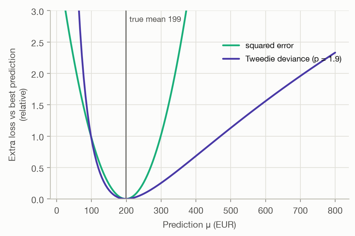
Both losses are minimized at the true mean, so both reward predicting the mean.
They differ in how they punish a miss: squared error is symmetric, so
predicting 0 costs as much as predicting double the mean. The deviance
punishes under-prediction much harder, because a low $\mu$ claims that large
outcomes are nearly impossible.
## D²: the deviance version of R²
Like R², the **fraction of deviance explained** compares a model with the Null
model:
$$
D^2 = 1 - \frac{\sum_i w_i\, d(y_i, \hat\mu_i)}{\sum_i w_i\, d(y_i, \bar y)}.
$$
With $p = 0$ it equals R². Like R², it is 0 for the Null model, can be
negative for a model worse than the mean, and can't be compared across
datasets.
```{python}
#| label: tbl-deviance
#| tbl-cap: "Exposure-weighted Tweedie deviance (p = 1.9) and D² on the test set."
#| code-fold: false
pd.DataFrame({
    m: pd.concat([deviance_metrics(y, p[m], p["Null"], w, TWEEDIE_POWER),
                  regression_metrics(y, p[m], w)[["bias", "R²"]]])
    for m in ("Null", "GLM", "GBM")
}).round(4)
```
```{python}
#| include: false
d2 = {m: deviance_metrics(y, p[m], p["Null"], w, TWEEDIE_POWER)["D²"] for m in ("GLM", "GBM")}
r2 = {m: regression_metrics(y, p[m], w)["R²"] for m in ("GLM", "GBM")}
```
Compared with R², the deviance gives a clearer picture:
- Both models explain about `{python} f"{d2['GBM']:.1%}"` of the deviance,
roughly **`{python} f"{d2['GBM'] / r2['GBM']:.0f}"` times their R²**
(`{python} f"{r2['GBM']:.2%}"` for the GBM): R² was drowned out by a few
huge claims.
- The GBM is slightly ahead of the GLM (`{python} f"{d2['GBM']:.2%}"` against
`{python} f"{d2['GLM']:.2%}"`). Whether a difference this small is real, and
not test-set noise, is a question for the [model-comparison page](../comparison/model-comparison.qmd).
### Is a D² this small good?
Yes: values like this are normal for individual insurance outcomes. Whether a
given policy has a claim this year is mostly chance, and no model can predict
chance. A pricing model's job isn't to predict *which* policy will claim but
to **separate low risks from high risks**. That ability shows up clearly in
ranking and segmentation tools (Lorenz curves, Gini, lift and double lift
charts), which barely react to the noise that dominates individual-level
metrics. They are covered on the [next page](lift-lorenz.qmd).
## Choosing the power
The deviance depends on $p$, and models can rank differently under different
powers. A quick sensitivity check:
```{python}
#| label: tbl-power
#| tbl-cap: "D² of each model under different Tweedie powers."
pd.DataFrame({
    f"p = {pw}": {m: deviance_metrics(y, p[m], p["Null"], w, pw)["D²"] for m in ("GLM", "GBM")}
    for pw in (1.2, 1.5, 1.9)
}).round(4)
```
Here the GBM stays ahead under every power, but the *level* of D² changes a
lot with $p$. A D² is only meaningful together with the power it was computed
with. Pick $p$ to match the target, ideally the power used to train the model
or one estimated from the data, and keep it **fixed** when comparing models.
If the ranking of models flips between plausible powers, neither model is
clearly better.
::: {.callout-note}
## A note on weights
Pure premium is a rate per policy-year, so a policy observed for a week gives a
very noisy rate. Weighting each policy's deviance by its exposure gives a
one-week policy 1/52 of the weight of a full-year policy, consistent with how
the models were fitted. Unweighted metrics would be dominated by short policies
with extreme rates.
:::
## Takeaways
- The **deviance** is the error measure that matches the target's
distribution, and it's what GLMs and GBMs actually minimize.
- For insurance targets use **Tweedie** (pure premium), **Poisson** (frequency)
or **Gamma** (severity) deviance, with exposure or claim-count weights.
- **D²** is the fraction of the Null model's deviance explained. Small values
are normal when outcomes are mostly chance.
- When individual outcomes are this noisy, **ranking and segmentation measures**
show a model's value better than any average error.